Compressing Neural Networks Using the Variational Information Bottleneck

This poster introduces our work about compressing neural networks in a less formal fashion to help you gain a big picture of our work. For a formal version, please check our paper. You can also refer to the arxiv version for more technical details including all the proofs and mathematics.

If you are not interested in the theoretical/mathematical part, you can skip the objective derivation part and the theoretical analysis part. Though mathematical derivations are unavoidable in the theoretical analysis part, I will try my best to make it as simple as possible and give you an intuitive sense.

2. Background

Though deep learning is very successful in many application domains, it is also well-known that most of the popular networks are over-parameterized. The consequence of over-parameterization is often three-fold:

Unnecessarily large model size,
Computational cost,
Run-time memory footprint.

In this work, we try to compress the network in all the three aspects. Basically, the proposed method is a pruning method (check related work for other methods). We have an over-parameterized model. Then we use some kinds of regularization to prune the original model and obtain a much smaller one. In the literature, there are two kinds of pruning methods. The first one only prunes weight connections, as shown in Figure 1 while the second one prunes weight groups or neurons / filters, as shown in Figure 2.

Figure 1. Illustration of Pruning Weight Connections.

Figure 2. Illustration of Pruning Weight Groups / Neurons / Filters.

3. High Level Intuition

We first interpret feed forward networks as a Markov chain, as shown in Figure 3(a). The input is $x$ while the target output (usually the label) is $y$. The hidden layers are denoted as $h_1, h_2, ..., h_L$ where $L$ is the number of layers. Sometimes we also denote the input layer as $h_0$ for convenience. The $i$-th layer defines the probability distribution $p(h_i|h_{i-1})$. If this distribution becomes a Dirac-delta function, then the network becomes deterministic. In the proposed model, we consider non-degenerate distributions of $p(h_i|h_{i-1})$. The last layer approximates $p(y|h_L)$ via some tractable alternative $p(\hat{y}|h_L)$. In the network, each layer extracts information from its previous layer. The last layer uses the information it extracted to give the prediction. Intuitively speaking, the more useful information it extracted, the higher predicting accuracy it will be.

Figure 3.

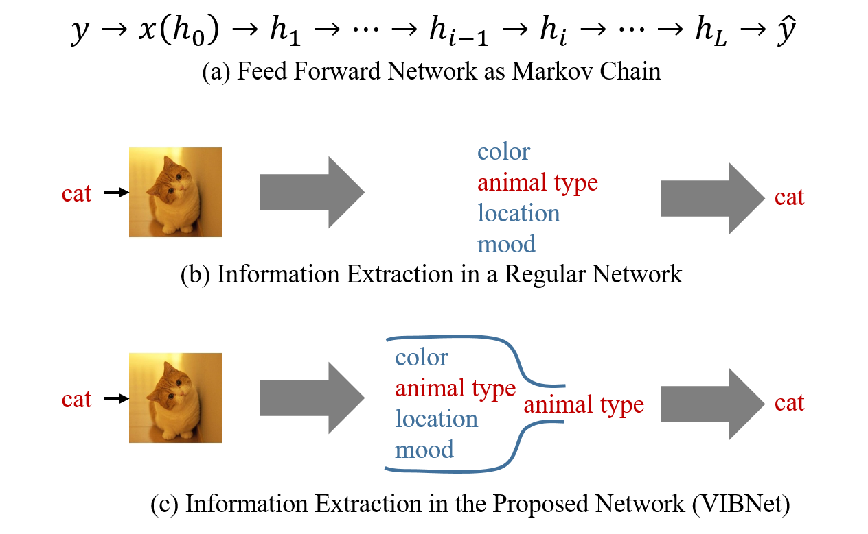
We take Figure 3(b) an example. We have a label ($y$) "cat" and an input image ($x$). The hidden layers extracts a lot of information about the input image. For example, the color, the animal type, the location, the moode and so on. The output layer tries to use these information to output the animal type i.e. "cat". However, we can see most of the information extracted by the hidden layers is actually irrelevant to our task, which means there is a huge room for us to compress the network. Our high level intuition to compress the network is

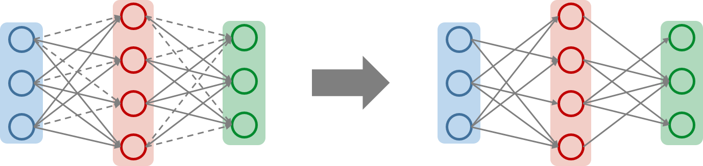
Only extract relevant information for our task;
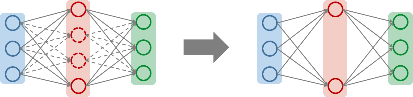
Aggregate the relevant information to part of the network such that the rest part of the network can be pruned.

For the first intuition, we use an information bottleneck, which is first proposed by Tishby et al. (2000), to enforce each layer only extracting the relevant information about the task. That is

Maximize the mutual information between $h_i$ and $y$, i.e. $I(h_i; y)$;
Minimize the mutual information between $h_i$ and $h_{i-1}$, i.e. $I(h_i; h_{i-1})$.

So the layer-wise energy function becomes $$\mathcal{L}_i=\gamma_iI(h_i;h_{i-1})-I(h_i;y),$$ where $\gamma_i$ is a hyper parameter that controls the bottleneck strength. If a layer $h_i$ extracts some irrelevant information about $y$, we can decrease the energy $\mathcal{L}_i$ by removing this part of information, which will not change $I(h_i;y)$ but decrease $I(h_i;h_{i-1})$. As shown in Figure 3(c), the proposed method uses an information bottleneck to filter out the irrelevant information and only let the relevant part to go through. We aggregate the relevant information to only part of the network by using a sparse-promote prior on each hidden neurons. You can see the details in the objective derivation section. If you are not interested in mathematics, you can directly go to the end of the next section and check the final practical objective function and the network structure.

4. Objective Derivation

4.1 Upper Bound

The layer-wise energy defined above is often intractable in a deep neural network. So instead of optimizing it directly, we optimize an upper bound of it. Basically we use variational distributions which can be defined by the network to approximate the true distributions and obtain the upper bound according to Jensen's inequalicy. Take the mutual information between $h_i$ and $h_{i-1}$ for example, we have $$\begin{align}I(h_i;h_{i-1}) &= \int p(h_i,h_{i-1}) \log \frac{p(h_i,h_{i-1})}{p(h_i)p(h_{i-1})} dh_i dh_{i-1} \\ &= \int p(h_{i-1}) p(h_i|h_{i-1}) \log \frac{p(h_i|h_{i-1})}{p(h_i)} dh_i dh_{i-1} \\ &\le \mathbb{E}_{h_{i-1}\sim p(h_{i-1})} \left[ \mathbb{KL}\left[ p(h_i|h_{i-1}) || q(h_i) \right] \right]. \end{align}$$ The inequality comes from Jesen's inequality by replacing $p(h_i)$ with a variational distribution $q(h_i)$ and it holds for any kind of distribution. The final upper bound is $$\begin{align} \tilde{\mathcal{L}}_i = & \gamma_i \mathbb{E}_{\{x,y\}\sim\mathcal{D}, h_i \sim p(h_i|x)} \left[ \mathbb{KL}\left[ p(h_i|h_{i-1}) || q(h_i) \right] \right] \\ & -\mathbb{E}_{\{x,y\}\sim\mathcal{D}, h\sim p(h|x)} \left[ \log q(y|h_L) \right], \end{align}$$ where $\mathcal{D}$ is the data distribution and $h$ stands for the union of $h_1, h_2, ..., h_L$.

4.2 Parameterization

We then need to specify the parameterization of the probability distributions in the upper bound. More specifically, we need to parameterize three distributions: $p(h_i|h_{i-1})$, $q(h_i)$ and $q(y|h_L)$. For other distributions in the upper bound, $\mathcal{D}$ is the groundtruth distribution of the given dataset, $p(h_i|x)$ (or $p(h_i|h_0)$) can be written as the marginalization of $\Pi_{j=1}^{i} p(h_j|h_{j-1})$ while $p(h|x)$ can be simply written as $\Pi_{j=1}^{L} p(h_j|h_{j-1})$.

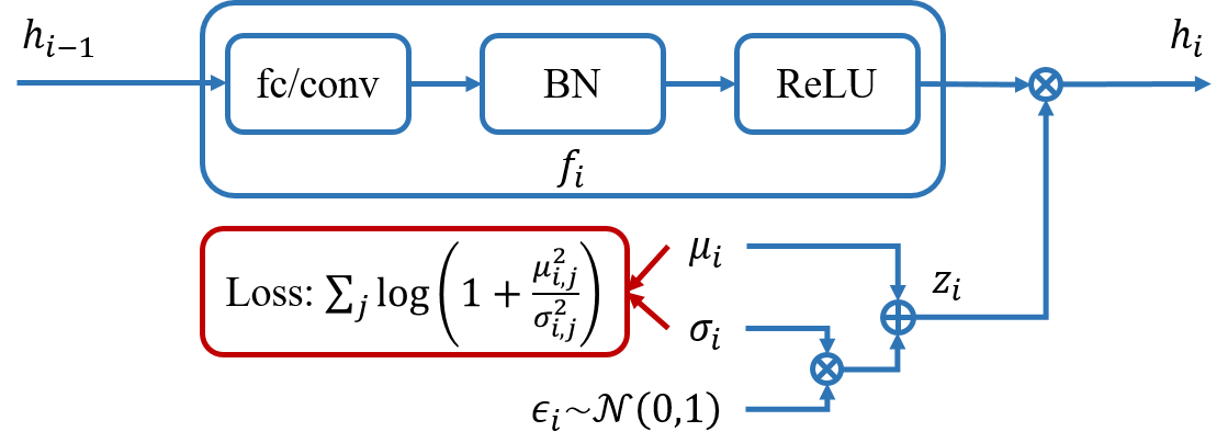
The parameterization of $q(y|h_L)$ is quite straight-forward. It is a multinomial distribution for a classification task and produces a cross-entropy loss. For a regression task, it becomes a Gaussian distribution and gives a Euclidean loss. We define both $p(h_i|h_{i-1})$ and $q(h_i)$ as Gaussian distributions as follows $$\begin{align} p(h_i|h_{i-1}) &\sim \mathcal{N} \left(f_i(h_{i-1})\odot\mu_i, \text{diag}\left[ f_i(h_{i-1})^2\odot\sigma_i^2 \right] \right), \\ q(h_i) &\sim \mathcal{N} \left( 0, \text{diag}\left[ \xi_i \right] \right). \end{align}$$ Here $f_i(\cdot)$ is a deterministic transformation. In practice, it is usually a concatenation of a fully connected / convolution layer, a batch normalization layer and an activation layer (see Figure 4). $\odot$ stands for element-wise product. $\mu_i$ and $\sigma_i$ are two free parameters which have the same dimension as the corresponding layer. If we fix $\mu_i$ to be $1$ and $\sigma_i$ to be $0$, then $p(h_i|h_{i-1})$ degenerates to a Dirac-delta function spiking at $f_i(h_{i-1})$ and the network becomes a regular one.

$q(h_i)$ is also a Gaussian distribution with zero mean and a learnable covariance $\xi_i$. Such a prior can help promote the sparsity and aggregate the information to part of the neurons rather than distribute the information to all the neurons [2]. For example, if the covariance of the $j$-th dimension ($\xi_{i,j}$) becomes $0$, the corresponding $p(h_{i,j}|h_{i-1})$ will also be a Dirac-delta function spiking at $0$ otherwise it will produce an infinite large KL divergence. Intuitively speaking that dimension can be safely removed.

4.3 Approximation

Since both $p(h_i|h_{i-1})$ and $q(h_i)$ are Gaussian distributions, the KL divergence between them can be written in a closed form. Moreover, we can optimize $\xi_i$ out of the model rather than learn it inside the network. After some simple derivations, we obtain $$\begin{align} & \inf_{\xi_i \succ 0} \mathbb{E}_{h_{i-1} \sim p(h_{i-1})} \left[ \mathbb{KL} \left[ p(h_i|h_{i-1}) || q(h_i) \right] \right] \\ \equiv & \sum_j \left[ \log\left(1+\frac{\mu_{i,j}^2}{\sigma_{i,j}^2}\right) + \psi_{i,j} \right], \end{align}$$ where $\psi_{i,j}$ is a non-negative value. For the sake of optimization convenience, we omit this term and our final objective becomes $$\tilde{\mathcal{L}} = \sum_i \gamma_i \sum_j \log\left(1+\frac{\mu_{i,j}^2}{\sigma_{i,j}^2}\right) -L \mathbb{E}_{\{x,y\}\sim\mathcal{D},h\sim p(h|x)} \left[ \log q(y|h_L) \right].$$ This objective is composed of two terms: a regularization term that tries to compress the neural network and a data term that tries to fit the data distribution. More interestingly, the regularization is only related to the extra parameters $\mu_{i,j}$ and $\sigma_{i,j}$ but not related to the parameters in $f_i(\cdot)$, which makes the implementation much easier. The $i$-th layer structure is shown in Figure 4.

Figure 4. Network Structure of the $i$-th Layer.

5. Theoretical Analysis

6. Empirical Results

8. ICML 2018 Oral

Reference

[1] Tishby, N., Pereira, F. C., and Bialek, W. The information bottleneck method. arXiv:physics/0004057, 2000.
[2] Tipping M E. Sparse Bayesian learning and the relevance vector machine[J]. Journal of machine learning research, 2001, 1(Jun): 211-244.