Bin Dai
Ph.D. candidate
Institute for Advanced Study (IAS)
Tsinghua University (THU)
Contact: daib09physics@gmail.com
Tutorial on Variational Autoencoders
Variational autoencoder (VAE) is a popular generative model proposed recently [1][2]. This poster gives a simple explanation of VAE and is inspired by the tutorial[3]. I will start from the big picture of generative and go to the details of VAE step by step. Hope this poster makes sense to you.
1. Outline
2. Background
In the realm of machine learning, there are basically two kinds of models: the discriminative model and the generative model. Suppose we have an observable variable $X$ and a target variable $Y$. Usually $X$ can be the variable representing an input image and $Y$ stands for the label of the image. A discriminative model tries to predict the target $Y$ given the observed variable $X$. It models the conditional probability $p(Y|X=x)$. However, a generative model tries to learn how the data is generated given a certain target (or label) $Y=y$. In other words, it models the probability $p(X|Y=y)$. Sometimes even the target is not given. The model tries to capture the distribution of the observable variable $X$,
In a traditional generative model like latent Dirichlet allocation (LDA) [4], we usually design how the data is generated by hand. Take LDA for example, it tries to generates a bunch of documents. We first have a topic distribution. Each topic defines a probability distribution over the words. Such a generation procedure is designed by hand. These traditional generative models have at least three draw-backs:
- Strong assumptions about the structure of the data;
- Severe approximations which lead to suboptimal problems;
- Computational expensive inference like MCMC.
2. VAE Model
2.1 Latent Variable Model
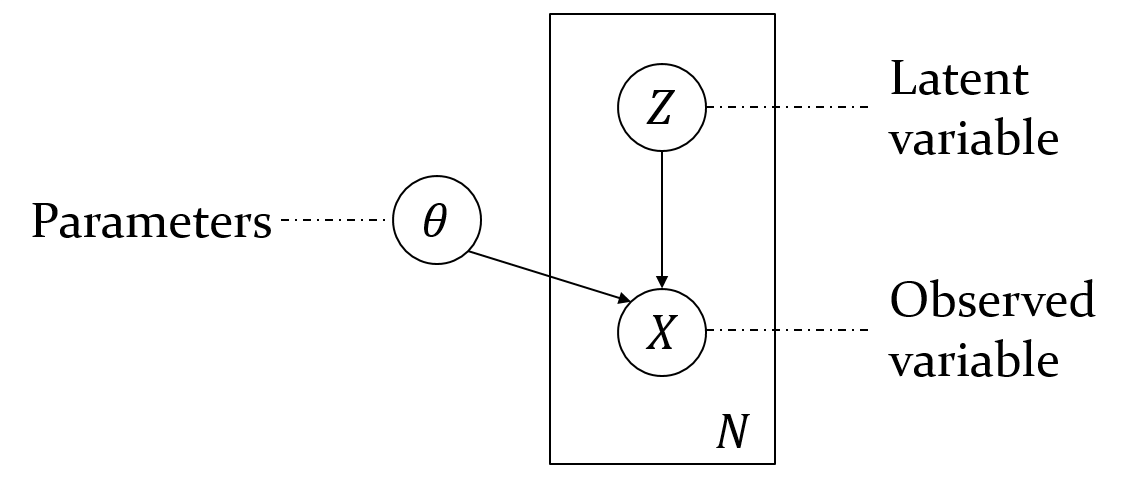
The graphical model of VAE is shown in Figure. 1. Assume there is a latent variable $Z$ that contains all the information needed to generate a sample. For example, for a digit generation task, one dimension of $Z$ can represent what the digit is while another dimension can stand for the font style. With the information given by the latent variable, we also need to know how to generate the digit, which is given by the parameter $\theta$. Given a certain $Z=z$, we can obtain the observed variable $X=x$. The final goal of the model is to maximize the log likelihood $$\log p_\theta(x) = \log \int p_\theta(x|z) p(z) dz.$$
2.2 Derivation of the Objective Function
Unfortunately, the integration in the log likelihood is usually intractable. To optimize the parameter $\theta$ in the log likelihood, we have to make some compromise. So we optimize an evidence lower bound (ELBO) of the log likelihood in practice. The lower bound is derived as the following $$\begin{align} \log \int p_\theta(x|z) p(z) dz &~~=~~ \log \int q_\phi(z|x) \frac{p_\theta(x|z)p(z)}{q_\phi(z|x)} dz \\ &~~ \le \int q_\phi(z|x) \log \frac{p_\theta(x|z)p(z)}{q_\phi(z|x)} dz \\ &~~ = -\mathbb{KL}\left[ q_\phi(z|x) || p(z) \right] + \mathbb{E}_{z\sim q_\phi(z|x)}\left[ \log p_\theta(x|z) \right]. \end{align} $$ The second inequality comes from Jensen's inequality. $q_\phi(z|x)$ can be any kind of distributions. $\mathbb{KL}[\cdot||\cdot]$ stands for KL divergence. This objective is composed of two terms, the first regularization term, which tries to regularize the distribution of $z$, and the second data fit term, which tries to fit the data distribution.
In this objective, we have $q_\phi(z|x)$ which projects $x$ to a distribution in the latent space. And we also have $p_\theta(z|x)$ which projects $z$ the a distribution in the observed space. That's why we call the model variational autoencoder. $q_\phi(z|x)$ is the encoder parameterized by $\phi$ and $p_\theta(x|z)$ is the decoder parameterized by $\theta$.
2.3 Parameterization of the Distributions
By far we have derived the objective function. Then we need to specifically define the parameterization of the distributions in the objective. The definition of the prior $p(z)$ is quite simple. We let it be a normal Gaussian distribution $\mathcal{N}(0, I)$. Each dimension of $z$ stands for a kind of attribute. However, we do not know what exactly that attribute is. The approximate posterior is also defined as a Gaussian distribution for simplicity. Of course such a choice is not necessary and there are other works using a more flexible distribution. For computation convenience, the Gaussian distribution is diagonal,
The distribution $p_\theta(x|z)$ is also defined as a Gaussian distribution $\mathcal{N}(\mu_x,\lambda I)$. Sometimes $\lambda$ is fixed as $1$ and $\log p_\theta(x|z)$ becomes a Euclidean loss. We can also set the covariance as $\text{diag}[\sigma_x]$, just like the covariance in the encoder. With these specific parameterization, the final objective function becomes $$\begin{align} \mathcal{L}(\theta,\phi) \triangleq & -\sum_i \frac{1}{2} \left( \mu_{z,i}^2 + \sigma_{z,i}^2 - \log\sigma_{z,i} - 1 \right) \\ & - \frac{1}{L} \sum_{l} \left( \frac{||x-\mu_x^{(l)}||_2^2}{2\lambda} + \frac{d}{2}\log\lambda \right), \end{align}$$ where $d$ is the dimension of $x$. We use a Mento carlo method to approximate the term $\mathbb{E}_{q_\phi(z|x)}[\log p_\theta(x|z)]$. $L$ samples $z^{(l)}$ are drawn from the distribution $q_\phi(z|x)$ and fed into the decoder. The corresponding decoder mean are $\mu_x^{(l)}$.
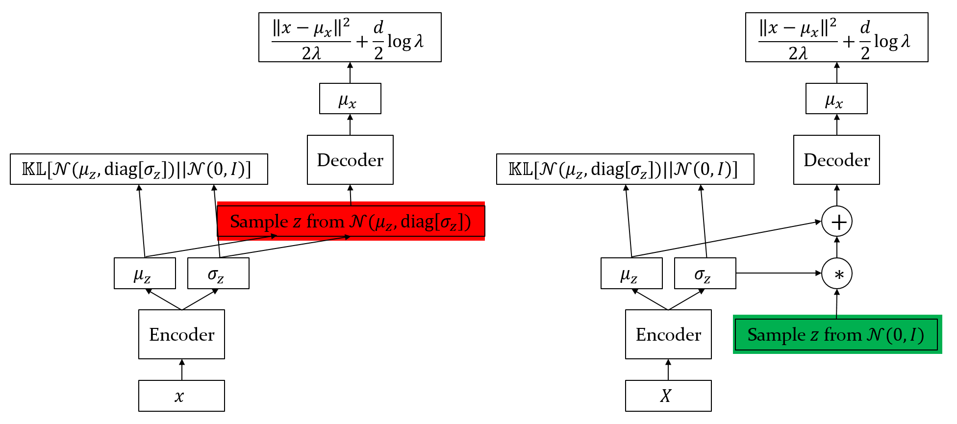
2.4 Reparameterization Trick and Network Structure
With the previous derivations, the network structure is like Figure 2(left). However, one issue with this structure is that the gradient from the data fit term is blocked by the sampling operator such that it cannot propagate back to the encoder. As a result, the KL term will force the encoder to learn a trivial distribution,
Reference
[1] Kingma D P, Welling M. Auto-encoding variational bayes[J]. arXiv preprint arXiv:1312.6114, 2013.
[2] Rezende D J, Mohamed S, Wierstra D. Stochastic backpropagation and approximate inference in deep generative models[J]. arXiv preprint arXiv:1401.4082, 2014.
[3] Doersch C. Tutorial on variational autoencoders[J]. arXiv preprint arXiv:1606.05908, 2016.
[4] Blei D M, Ng A Y, Jordan M I. Latent dirichlet allocation[J]. Journal of machine Learning research, 2003, 3(Jan): 993-1022.